
Long-Term Capital Management (LTCM) was a hedge fund founded in the early 1990s by former Salomon Brothers trader, John Meriwether and led by two Nobel Prize Laureates, Myron Scholes and Robert C. Merton. At LTCM, their team used complex mathematical models to derive trading profits from leveraged investments until their ultimate collapse in 1998.
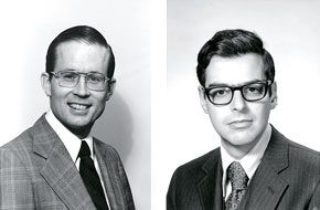
You may have heard these names before - they are the same Scholes and Merton from the Black-Scholes-Merton model. Their models are still used today by millions of economists and financial professionals primarily to value "options" - a type of financial instrument with value derived from underlying securities (such as stocks). You may encounter options if you work at a startup or trade call or put options on a public exchange.
The story of LTCM is fascinating one and also a cautionary tale for applying mathematics in finance.
Gaining steam
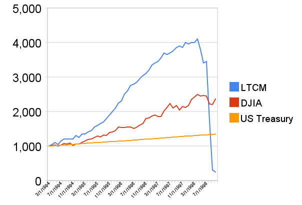
Having a team of some of the most connected and brightest minds in finance meant LTCM was able to easily raise funds on Wall Street. LTCM's founders had stellar reputations and investors were honored to participate. Most were already well versed in their contributions to finance. In a matter of months they were able to raise more than $3 billion and that grew substantially as LTCM outperformed the S&P500 consistently for the first three years. Much of LTCM's capital was composed of funds from the same financial professionals with whom it traded.
Working out of an office in Greenwich, Connecticut, LTCM kept their strategies secret. Investors paid $10 million or more to get into the fund. They were not permitted to take the money out for three years or inquire about LTCM investing strategies.
Most of LTCM's investment strategies were based upon hedging against a predictable range of volatility in foreign currencies and bonds. Due to the small spread in arbitrage opportunities, LTCM had to leverage itself highly to make money. At their peak, LTCM had more than $100 billion under management with leveraged investments rumored to be more than $1 trillion.
The Collapse and Bailout
In August of 1998, Russia's declining productivity, high fiscal deficit and unfavorable exchange rates reached a critical point. As a result, the Russian government and the Russian Central Bank devalued their currency and defaulted on its debt. This event and the effects that rippled across financial markets worldwide were well beyond the normal range that LTCM had estimated. LTCM's investments started to crumble.
In 1998, The Federal Reserve Bank of New York organized a bailout of just over $3.5 billion by major creditors to avoid a wider collapse in the financial markets. Since so many banks and pension funds had invested in LTCM, its problems threatened to push most of them to near bankruptcy.
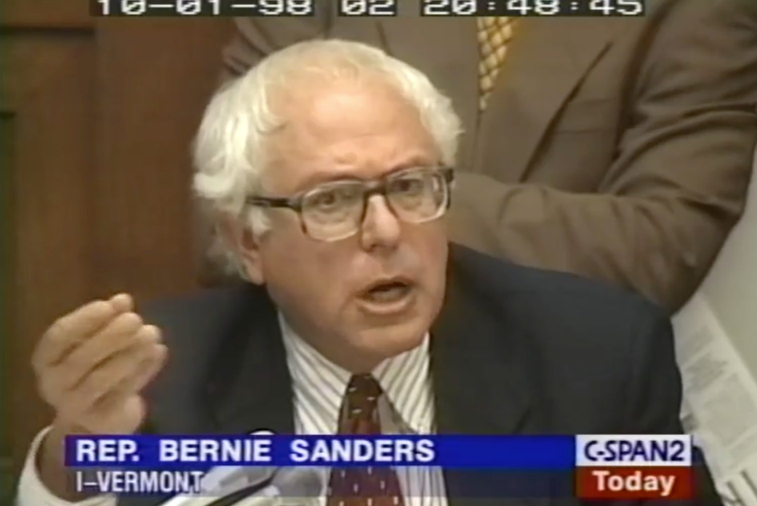
The demise of LTCM was highly publicized and subsequently analyzed in detail. During bailout hearings, LTCM was criticized for reckless behavior which amounted to the equivalent of gambling. A small group of people's investments threatened global economic stability.
History does not always predict the future
Many of LTCM's many strategies were built on the premise that the price difference between two types of securities (mostly fixed income ex. bonds) would "converge" around its historical mean. Their swap spread strategy was believed to be "mean reverting" and would work unless the difference between two prices exceeded acceptable and unlikely thresholds. The 1998 Russian financial crisis obliterated LTCM's model thresholds and triggered rapid trading losses.
LTCM strategies were once compared to "vacuuming up nickels" from inefficiencies in markets. After LTCM went bust, these same strategies were compared to "picking up pennies in front of a steamroller". It is a very clear example of the classic lesson that history does not always predict the future.
Mimicking LTCM
It is easy to find additional reading material on LTCM including a few entertaining documentaries. If you want to learn more about LTCM I can recommend "When Genius Failed: The Rise and Fall of Long-Term Capital Management" by Roger Lowenstein or the 1999 BBC Horizons Documentary "The Midas Formula".
I wanted to provide enough background to introduce an algorithmic trading strategy that mimics the same strategies used by LTCM.
Fair warning
Here is where things get technical. Some statistics knowledge is needed as well as familiarity with market microstructure and finance in general. A disclaimer is that I would not recommend deploying this strategy but you will also find that it is difficult to succeed in this without commercial discounts on trading fees and reduced slippage.
Mean reversion strategy: "Pairs" Trading
Because of LTCM, mean reversion strategies are well-known and infamous in algorithmic trading and trading in general. One of the more popular strategies is commonly referred to as "pairs" trading and is the one I will be sharing how to perform effectively while understanding what is happening.
A pairs trade is a market neutral trading strategy where trading profit can be obtained in any market condition - independent of whether a security's price trend is increasing, decreasing, or horizontal. This strategy is often categorized as statistical arbitrage and like with LTCM, it relies on "convergence" and "mean reverting" of price differences.
When you hear this it is common to think that this is the proverbial holy grail of trading strategies. "I can trade without estimating which direction a stock will go!" Just keep in mind the lessons from LTCM throughout.
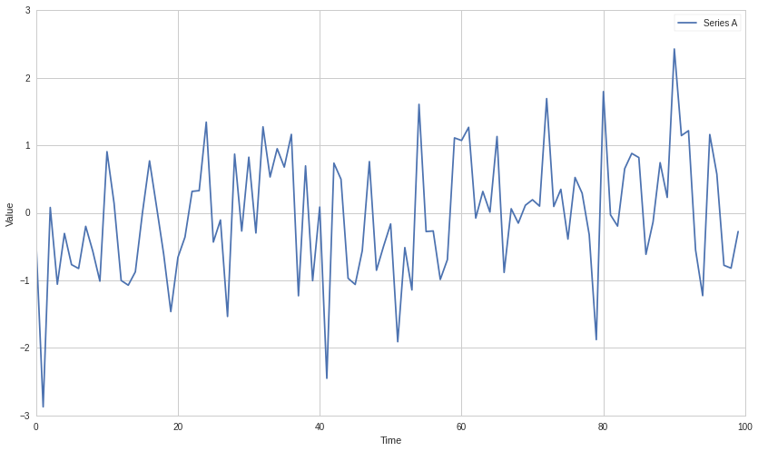
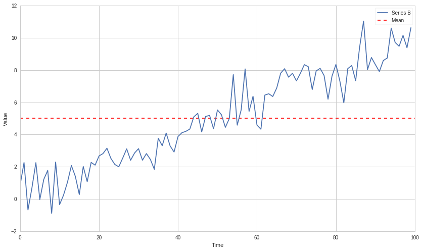
Stationary time series
A stationary time series is one whose statistical properties such as mean, variance, autocorrelation, etc. are all constant over time. As part of this strategy, we want the price differences of two securities to revert around a mean. So naturally, the price differences over time should be stationary.
The default null hypothesis is that the time series is non-stationary. To test this null hypothesis you could use an "Augmented dickey fuller"(ADF) test. This tests the null hypothesis that a unit root is present in a time series sample. We can then use a cut-off p-value to reject the null hypothesis. ie. determine if the time series is "likely stationary".
If we can take one price series and some other price series with a stationary spread and then buy one and short the other this effectively acts as hedge and will create trading profit as the prices revert to the mean. For example, if we bought $100 dollars worth of a loser (L) and shorted $100 dollars worth of winner (W), and when their prices converged we could sell L for $110, and pay $90 for W. In the end, we made $20.
Stop losses are recommended for when the differences exceed a preset standard deviation σ (sigma). Lack of effective stop losses is they key reason that LTCM failed. It should become very clear that this type of strategy is particularly dangerous if the time series of price differences is non-stationary. If the price differences never return to the mean, profits will never be realized.
The goal then becomes finding two (or more) securities whose price differences are stationary over time. We will get into how to test for stationarity later. Although I mentioned that history does not predict the future, without it there is no evidence to suggest mean reversion.
Finding pairs
Unless there's a reasonable economic basis for why the randomness inherent in one time series would explain the randomness of another time series well then we have no reason to believe that it's going to continue to be so. Price differences need to remain stationary over time so trading profit can be realized over time.
Explaining the non stationarity of some time series with the non stationarity of some other time series is a very difficult relationship to explain and it's also a very difficult relationship to find. Maybe two companies that are publicly traded are dependent on each other or on some underlying economic indicator. Maybe there is a joint relationship in some sector or maybe one company is attempting to copy a competitor.
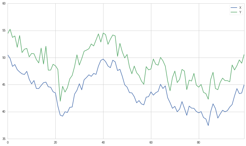
We want to start with some reasonable economic basis for the pair and in trying to find this relationship we can narrow the search space in hopes that we can actually find a legitimate relationship.
With the key assumption that returns are normally distributed, it's hard enough to find one stationary return time series unless you take a particular year so it's going to be significantly harder to find a pair of time series that are stationary together - that's a weird and sort of subtle relationship.
A good start is evaluating whether two securities are cointegrated.
Cointegration
This should not be confused with correlation. Correlation and cointegration, while theoretically similar, are not the same. Cointegration focuses on the spread between the two time series whereas correlation focuses on their direction in relation to each other. There are many ways to test for cointegration and it is convenient that with most tests, if a pair is likely cointegrated it is also likely stationary.
In practice a common way to do this for pairs of time series is to use linear regression to estimate β in the following model.
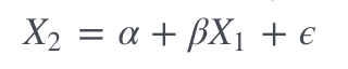
The idea is that if the two are cointegrated we can remove X2's depedency on X1, leaving behind stationary noise. The combination X2 − βX1 = α + ϵ should be stationary.
It is worth repeating that you should not assume that because some set of securities have passed a cointegration test historically, they will continue to remain cointegrated.
Putting it all together
This strategy is often deployed with diversification. A quant would normally identify many pairs of securities they hypothesize are pairs and as long as more than half of the pairs are successful, the strategy will work. As mentioned, stop losses are key and because spreads are small in today's markets it is difficult to realize substantial profits without significant capital and low fees/slippage. If you want to try it out programmatically using python I would recommend giving "Quantopian" a try. They have a built-in backtesting solution and some of the information gathered here is directly from that platform.